Introduction
What quantum computing changes, superposition, entanglement, interference, physical anchors, history, and the book’s roadmap.
Volume I · Foundations · A graduate problem book with full solutions
Can you derive the result—not merely recognize it?
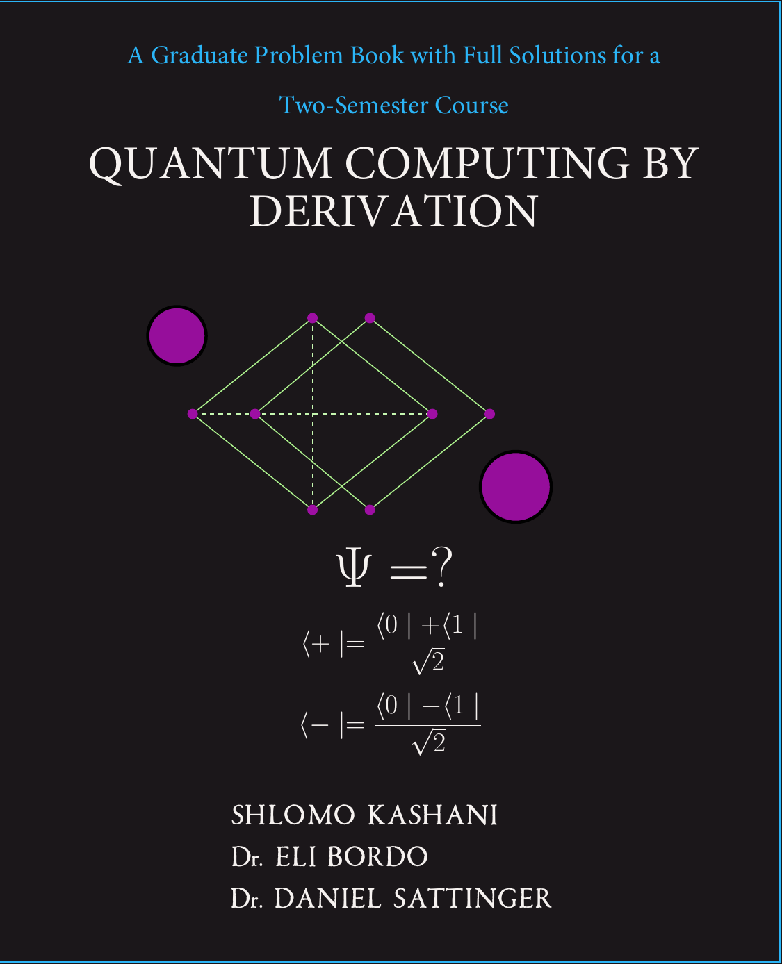
Volume I of Quantum Computing by Derivation is a problem-driven study and reference book for graduate students, instructors, researchers, and engineers who need more than an introductory survey.
It pairs mathematically explicit derivations with an entrance mock examination, worked problem banks, circuit practice, and structured verification. The aim is active fluency: knowing how a result is built, when it applies, and how to check it.
Volume I contains thirteen chapters, beginning with an introduction and entrance mock examination before developing the mathematical and physical foundations of quantum computing.
What quantum computing changes, superposition, entanglement, interference, physical anchors, history, and the book’s roadmap.
A rules-based diagnostic examination with problems and complete solutions.
Kets, bras, inner and outer products, adjoints, completeness, basis changes, operator reconstruction, and continuous bases.
Tensor products, Bell states, traces, commutators, vectors, norms, projectors, eigenvalues, and eigenvectors.
Spinors, superposition, normalization, measurement, eigenbases, time evolution, uncertainty, density matrices, and Bloch-sphere geometry.
Pauli identities, projector representations, basis decomposition, commutation relations, exponentials, rotations, and gate conjugation.
Single- and two-qubit expectation values, variance, uncertainty, Born-rule examples, shot-based estimators, and Hamiltonian checks.
Single-, two-, and multi-qubit gates, unitarity, rotations, circuit identities, optical gates, interferometers, and controlled operations.
Purity, partial traces, entanglement measures, Kraus operators, Choi representations, state distances, entropy, correlations, and open systems.
Bell and GHZ preparation, measurement structure, reduced states, entropy, teleportation, swapping, separability, and CHSH checks.
Spectra, conservation, exchange, singlet states, coupled-spin dynamics, chain simulation, and transverse-field Ising problems.
Unitary evolution, Pauli exponentials, Larmor precession, Lie–Trotter and Suzuki formulas, accuracy targets, and slice counts.
The Stern–Gerlach experiment and the distinction between superposition and statistical mixture.
A practical appendix on measurement settings and expectation estimation for Pauli strings.
About the authors

Author
Shlomo Kashani builds production AI and quantum systems — and studies the high-stakes decisions that ride on them. He ships large language models, retrieval, and agentic AI, and works hands-on across the quantum stack: quantum machine learning (QML), quantum algorithm design, and high-performance circuit simulation. His academic formation spans Defence and Strategic Studies at Missouri State University, an M.Sc in Quantum Physics & Computing at Johns Hopkins University, and an M.Sc in Digital Signal Processing at Queen Mary, University of London.

Author
Dr. Eli Bordo is a physicist by training and a technology leader by profession. He received his Ph.D. in quantum and ultrafast optics from the Technion, Israel Institute of Technology, studying light at the scales where classical intuition begins to give way to quantum mechanics. Today, he leads R&D efforts across quantum technologies, photonics, and other emerging fields, with a particular interest in turning elegant physics into working technology.
Author
Biography forthcoming.
This section combines three detailed mock-exam questions with a full Hamiltonian-simulation example. Follow the Ising model from Pauli strings through Trotterization to an executable circuit, then try each question before opening its worked solution.
Extended mock-exam question · Hamiltonian simulation
Consider the two-qubit transverse-field Ising Hamiltonian
Your goal is to turn the formal time-evolution operator \(U(t)=e^{-iHt}\) into gates that a quantum processor can execute.
A complete solution connects four representations: the physical model, its Pauli strings, a controlled approximation to \(e^{-iHt}\), and the gates that a processor can actually execute. The Ising derivation and Heisenberg extension below carry that chain all the way through.
Full example A · Transverse-field Ising model
Physical model
The \(ZZ\) term rewards neighbouring spins that agree in the computational basis. The \(X\) term continuously rotates each spin away from that basis. Their competition produces nontrivial dynamics.
That local Pauli structure is exactly what lets us compile the evolution into one- and two-qubit gates.
Specialize to two qubits
Define \(H_{ZZ}=-JZZ\) and \(H_X=-h(XI+IX)\). Each word says exactly which local operator acts on each qubit.
Why approximation is needed
Because the layers do not commute, \(e^{-i(H_{ZZ}+H_X)t}\neq e^{-iH_Xt}e^{-iH_{ZZ}t}\) at finite time. An exact separation would discard commutator corrections.
Controlled product formula
The leading first-order global error scales as \(O(t^2/r)\), with its coefficient controlled by \(\lVert[H_{ZZ},H_X]\rVert\). More slices mean shorter steps and less ordering error.
Exact local compilation
The mappings are exact. Only the ordering of the noncommuting layers is approximate.
One first-order Trotter slice
The first CNOT stores \(Z_1Z_2\) parity on the target. \(R_z\) attaches the interaction phase. The second CNOT removes the temporary parity, and the two \(R_x\) gates apply the transverse field.
Full example B · Heisenberg spin chain
Open isotropic chain
Unlike the transverse-field Ising model, each neighbouring pair exchanges spin information through \(X\), \(Y\), and \(Z\). For \(N\ge3\), terms on overlapping bonds need not commute, so product formulas again provide a systematic gate construction.
First-order chain step
The three worked questions
Try each problem before opening its worked solution. Every solution keeps the intermediate vectors, matrices, algebra, and independent checks visible.
Sample 01 · Expectation values
Let
This is a single Pauli operator applied to a two-component state, worked out one row at a time.
Complex conjugation changes \(2i\) into \(-2i\). Therefore
The safest route is to calculate \(P|\psi\rangle\) first and only then multiply by \(\langle\psi|\). This keeps the row-by-column bookkeeping visible.
\(X\) swaps the amplitudes.
The factors of \(i\) cancel.
\(Z\) flips the \(|1\rangle\) sign.
Since \(Z^2=I\), \(\langle Z^2\rangle=1\):
Independently, \(p_0=1/5\), \(p_1=4/5\), \(\mu_Z=(+1)p_0+(-1)p_1=-3/5\), and \(\mathbb E[Z^2]=1\).
The Bloch vector \((0,4/5,-3/5)\) has unit length, independently confirming a pure state and consistent arithmetic.
Sample 02 · Dirac notation
Two normalized qubit states are
Taking a bra conjugates every coefficient: \(-i\mapsto+i\) and \(e^{i\pi/4}\mapsto e^{-i\pi/4}\).
The probability is the squared length of the component of \(|\psi\rangle\) along \(|\phi\rangle\), not the complex overlap itself.
Off-diagonal entries are conjugates.
One eigenvalue is one.
The other eigenvalue is zero.
Sample 09 · Entanglement
Consider the normalized two-qubit state
The equal outcomes are \(00\) and \(11\), so \(P(\text{equal bits})=2/3\). The probabilities sum to one.
It is real and symmetric.
Diagonal entries sum to one.
Both eigenvalues are positive.
The global state is pure but the reduced state is mixed. Therefore \(|\Psi\rangle\) is entangled.
The reduced-state entropy is approximately \(0.550\) bits: nonzero, but below the one ebit of a Bell state.
The manuscript makes basis order, notation, intermediate steps, and acceptance criteria visible. Solutions are not compressed into answer-key form; they are written so a reader can reconstruct the reasoning and locate an error.
“The result matters. The route to the result is what makes it reusable.”
Passive familiarity
Definitions and finished formulas can create a sense of recognition without testing whether the formalism can be retrieved and used.
Technical fluency
Worked derivations, problem banks, and computational checks make the reader choose a representation, carry the algebra, and test the result.
The progression runs from Dirac notation, linear algebra, and single-qubit systems to measurement, circuits, quantum information, entanglement, coupled spins, Hamiltonian dynamics, and quantum physics.
A derivation should survive more than one form of scrutiny.
Learn
Follow complete solutions with explicit notation, intermediate reasoning, and clearly stated assumptions.
Practise
Use chapter-aligned problem banks and the entrance mock examination for structured revision.
Verify
Reproduce analytical claims with computational checks and portable implementation guidance.
Book details
Kashani, Shlomo; Eli Bordo; and Daniel Sattinger.
Quantum Computing by Derivation. Volume I: Foundations.
A Graduate Problem Book with Full Solutions.
First edition, 2026.